


Technical Articles
10.05.21
Laser scanning – pretty pictures or High-Definition Mapping?
Part 2. FACT OR FICTION?
In the day and age of Fake News, it can often be hard to determine the truth. Without looking at the detail, headlines can be skewed to direct the audience to a particular conclusion. Everybody can sometimes be guilty of this to a degree, based on their bias and perspective. It only becomes an issue when blatantly distorting facts to mislead people.
In a previous blog, I discussed the popular perception that terrestrial laser scanners produce nothing more than ‘pretty pictures’ when considering their use for determining floor flatness spec compliance. I explained that using appropriate equipment in a tightly controlled process, it is possible to collect data of a sufficiently high quality to produce HD maps of the surface. These maps can then be used to determine conformity to specification. In this article, I will demonstrate using hard data what can be, and is achieved by Floor Dynamics on a daily basis.
Benchmarking
If you measure something using two different methods and get different answers, which one is correct? Or are they both wrong? The reality is all measurements have a degree of variation in repeatability, even using the same equipment and methodology. This variance is defined as uncertainty, which is an expression of the statistical dispersion of results. This is complex subject and for the purpose of this article, we shall accept that to quantify the quality of a measurement, it needs to be compared against a standard of agreed accuracy.
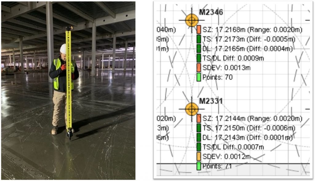
The Floor Dynamics process for producing HD maps uses multiple instruments to ensure the quality of the data. Fig. 1 shows an extract from a quality control report, comparing the value for a given spot collected using an engineering grade TSL with dual axis compensator, a 0.5” total station and a digital level with high precision invar staff.
The laser scanner positions are determined in order that sufficient data can be collected under its blind spot, from overlapping locations. Accurate registration of these individual scans within the control network is vital. Any issues with registration will be immediately apparent, when viewing the data within these dead zones.
Independent Testing
While Floor Dynamics’ processes provide validation of discreet points, we recently had the opportunity to take part in a test programme undertaken by the BCTA at the Building Performance Hub in High Wycombe.
Hexagon, the manufacturers of Leica instruments were asked to independently survey an area of floor measuring 25 x 1.5m using state-of-the-art laser trackers. A coordinate system was established using an ATS960 and a ‘benchmark’ area measured with the ATS960 and a T-Scan 5. The entire area of the test panel was then measured with an ATS600 Laser Tracker and cross referenced against the ‘benchmark’. A 50 x 50mm grid of levels was output, giving a total of 15,000 discreet points. Fig. 2 shows a coloured elevation map, often referred to as a heat map, of the data. Red is high. Blue is low.

Hexagon quote the ATS600 as having direct scanning guaranteed at up to 60 metres distance with metrology- grade accuracy to within 300 microns (when using SMRs). To compare, Floor Dynamics surveyed the test panel using a Leica P40 at 4 positions. This yielded 10.5 million lidar points that were then processed through our PellegoTM software to produce an equivalent 50 x 50mm grid of levels, the results of which are shown in fig. 3.

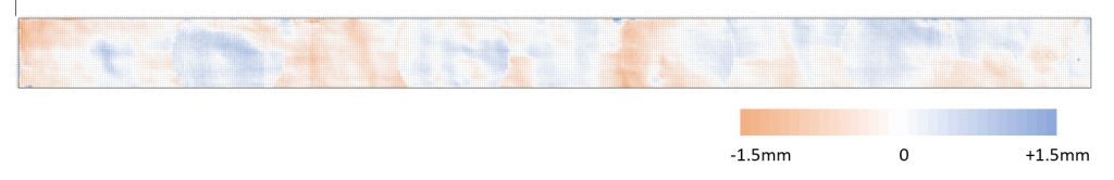
At first glance, these elevation maps are not far from identical. In fact, using other scanners and simpler processes yielded similar looking maps. In order to see any difference, the raw data from PellegoTM was subtracted from the ATS600 data to give a Z (height) value differential map, shown in fig.4.
Analysing the 15,000 individual points against each other yields the following spread, approximating to 1, 2 and 3 s:
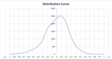
94.6% within +/- 0.5mm
99.5% within +/- 0.8mm
The reference slab had specific characteristics ground into the surface, in order test the surveying further. The 3D surface profile produced from the PellegoTM data set shown in fig.5, makes it much easier to visualise the contours compared to a heat map. Additionally, you can make out the tell-tale rings of the four scanner positions. The most visible, on the left of the image, is +0.3mm and is well within the uncertainty of 0.8mm stated.

The data set from the survey was then processed by PellegoTM to determine conformity to specification. Fig. 6 shows the location of errors that fall outside a rate in change of curvature of 6mm between two consecutive pairs of points, 300mm apart. Although calculated to a custom specification, this is essentially what we are measuring to with TR34 property F, or ASTM1155 property Ff. The beauty of these high-definition maps is that we can calculate not only along the grid but also perpendicular to the grid, across the entire surface. The colours represent the severity of the error.
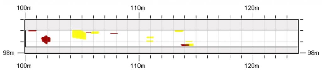

Interestingly, the two circles located to the right of the image, do not show as an error. This was additionally calculated manually and verified by direct inspection to confirm. All results show that this area falls just within specification.
This test programme, coupled with QA data cross-referenced on every project surveyed, demonstrates that Floor Dynamics quoted uncertainty of <0.8mm is not fabricated. The methodology is both robust and reliable and does not give rise to numerous positive or negative false errors. There is a caveat. As the 3D images show, this process is essentially photographing the entire surface, including anything on it. The floor must be clean at the time of scanning. Rubbish, piles of dirt, etc., will all be included and consequently, may lead to false positives (errors which are not there in reality). Larger obstacles could be removed during processing but then there is no data underneath. Best practice dictates cleaning.
Compounded Uncertainty
I have read and heard much criticism and scaremongering about the uncertainty of methodologies such as used by Floor Dynamics, especially in comparison to other measurement methods. ‘If an uncertainty of 0.8mm is quoted, then surely there must be a compounding effect when measuring rate of change errors. After all, there are 3 distinct points used in the calculation’. Theoretically, this is a valid argument. Unprocessed laser scanner data, selecting individual lidar points, could give rise to such issues. Laser scanners have a noise signature and a tolerance in terms of 3D position, horizontal and vertical accuracy. By taking approximately 200 individual readings in a 50 x 50mm cell, allows us to calculate the distribution of data. Comparing the Z value assigned to the cell with another instrument of known lower uncertainty, allows the determination of any bias in either measurement or registration. Fig 7. demonstrates the possible compounding impact of uncertainty in individual Z values when it comes to calculating a rate of change (curvature) error. In this example, the black lines represent the specification limit of 10mm. The red and green lines represent the upper and lower worst-case scenario of compounding uncertainties of 1mm. Theoretically, such a system could be reporting this error as 6mm (potentially a false negative) or 14mm (potentially a false positive).
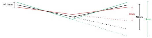
Fig 7. Potential effect of compounding uncertainties in calculating rate of change.
How other measurement systems stack up
During the process of understanding the limitations of terrestrial laser scanning technology, we have come to understand a great deal about other measurement devices used in the surveying of industrial floors. One piece of equipment that we have a lot of experience with is the walking electronic level, such as the FACE Dipstick or AXIOM 1155. Widely used for checking conformance against several standards, these devices are extremely accurate at measuring elevation difference between two discreet point, ie: the feet on the device, usually spaced at 300mm. Manufacturers quote accuracies in the order of 0.0125mm. While these devices are excellent, easy, and convenient to use, they do have drawbacks. Firstly, they are slow to use. This limits the amount of data that can be economically collected. They also have no idea where they are positioned in 3D space so are not reliable in reporting absolute elevation or reference to datum. Rolling versions of this type of equipment, while much quicker to use, can be prone to accumulating errors over distance.
When it comes to measuring to defined movement specifications, such as Concrete Society TR34, the options are very limited. The specification is written such that readings must be taken every 50mm along the wheel track. This dictates that a rolling floor profiler, more commonly known as a profileograph, is used. As the Floor Dynamics system plots data every 50mm, we are now able to directly compare against such equipment. It is important to point out that like laser scanners, not all profileographs are created equally.
On a recent project, where Floors Dynamics data was being questioned, we had the opportunity to do a direct comparison. While this is not a bullet proof scientific test, the results are interesting. It is possible to pinpoint with high precision a location on a Floor Dynamics HD map. This is repeatable due to tying into the established control network. Knowing exactly where a profileograph run is, cannot be said with such confidence. On sample profileograph runs of 150m in length, we plotted an equivalent trace from data that was within +/-100mm of the approximate profileograph position.
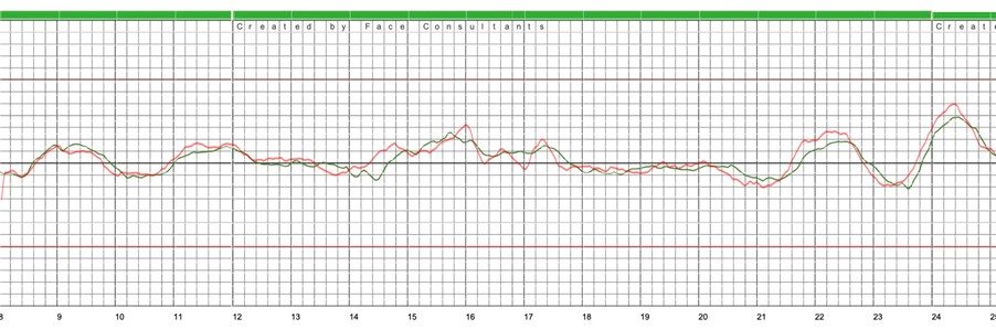
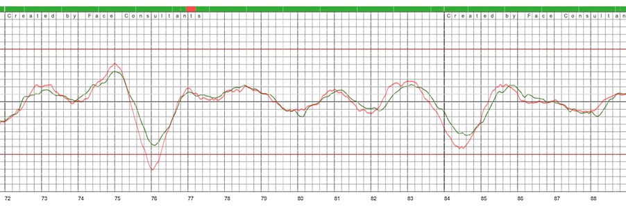
Fig. 8 plots the rolling elevation difference. The green trace is from the profileograph and the red, from PellegoTM. Considering that the traces may not be from exactly the same location, and that both methodologies have a degree of uncertainty, there is surprisingly good correlation. However, the end of the run, as shown in fig 9., is a different story
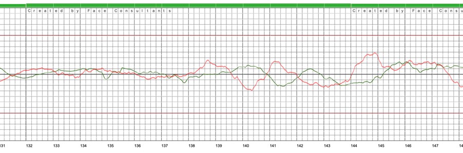
Stretching the PellegoTM data 1.2m on the X axis, once again the results are extremely close (Fig 10.). What this is suggesting is that profileograph has travelled 1.2m further over 150m. Several factors may explain this. Putting aside calibration, or even minor accumulation of material on the wheels, a rolling device is travelling up and down hill. It will naturally travel further than if it were on a perfectly flat surface. The grid of data output by PellegoTM is on a perfectly horizontal plan. This error may not be a problem if the data is broken up into smaller run lengths. This does explain however, why you cannot match two profileograph traces if measuring in one direction and then reversing direction, to take a second set of data.
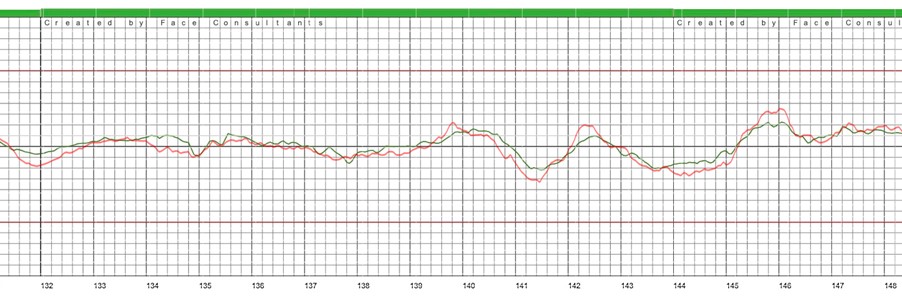
Somewhat more difficult to explain is the phenomena demonstrated in fig 11. Whenever there is very little change in elevation, eg: a constant slope or flat plane, there is very high agreement between the two data sets. However, when there is a rapid change in elevation, either in the positive or negative direction, there can be significant discrepancy. In the worst of cases, the profileograph is under-reporting the error by several millimetres. If the slope sensor response time is the issue, then running the profileograph slower would be expected to reduce this issue.
This is not the first time we have seen such a discrepancy. When constructing defined movement floors to TR34 DM1, not possessing a profileograph on site, our teams produce daily quality reports using a Dipstick. While this would conform to EN15620, which is essentially the same specification, TR34 prohibits the use of a Dipstick as it cannot take readings every 50mm. Invariably, the Dipstick survey will record worse results than a profileograph survey carried out by a 3rd party surveying company at project completion.
There could be many causes for this phenomenon. The most likely explanation is the response time of the slope sensor. With an electronic walking floor profiler, the operator must stop, allowing the slope sensor to settle, before the reading can be registered. It could be that with a rolling instrument, such as a profileograph, the sensor does not have time to reach its full reading before it reverses direction. As such, it would be under-reporting the error. It should be stressed that different manufacturers use different types of sensors.
Summary
Recognising that I have a bias, I have tried to be objective in the writing of this blog. There is a natural resistance to the introduction of disruptive technology. The only way to make an informed decision is based on data. The longer the debate persists, the more detail is being discovered. Not only in confirmation of new technology but also in the limitations of traditional methods. Ultimately, is the data able to yield sufficiently high-quality information on which to make decisions? In the world of automated logistics facilities, Floor Dynamics is increasingly demonstrating the value of mapping the entire floor surface, not just taking a statistical sample. For facilities employing robotics, consistent quality surface characteristics are required. Understanding if and where an area of floor needs remedial grinding, requires close co-operation between the various stakeholders of the construction process. The way in which data is presented and interpreted can cause confusion. Where an error is, is not where you need to grind. This is a whole other topic which I shall cover in a future post.
Andrew Keen
7th May 2021
Chief Services Office – RCR Industrial Flooring Group